Mechanics of Continua and Structures
Non-dimensionalization
Euclidean point space
We take that the world we live is a Euclidean point space, which we denote as $\mathcal{E}$. Thus, all the particles, rigid bodies, and continua we discuss in this course live, move, collide with each other, etc. in $\mathcal{E}$. We denote the points in $\mathcal{E}$ as $x$, $p$, etc., which if you recall is how we denote points in regular geometry.
We denote material particles, and collections of material particles, such as rigid bodies, as $\mathcal{X}$, $\mathcal{B}$, etc.
The reason we call $\mathcal{E}$ a point space and not a vector space is that for a set to be considered a vector space, it is necessary that we be able to add any two elements belonging to that set – and it does not make much sense to add points in $\mathcal{E}$. Think about the statement “add the floor’s northeast corner to its southeast corner.”
However, it does makes sense to measure the distance between points in $\mathcal{E}$. That is, it makes sense to make the statement “make the sofa’s width equal to the distance between the floor’s northeast corner and its southeast corner.” To be precise $\mathcal{E}$ is what we call a “metric space,” i.e., a set in which the notion of distance is well defined between any two of the set’s elements.
Euclidean vector space.
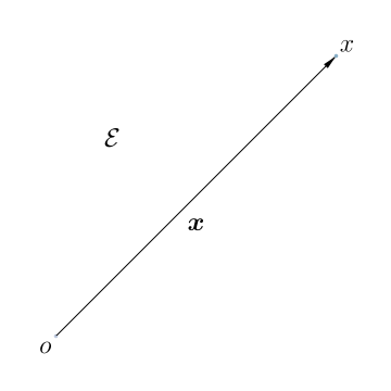
It also makes sense to talk about taking the shortest route to travel between two points in $\mathcal{E}$. Say $o$ (which, not surprisingly, we call the origin of $\mathcal{E}$) and $x$ are two points in $\mathcal{E}$. The shortest route to travel from $o$ to $x$ is well defined. It is marked as $\u{x}$ in the figure above.
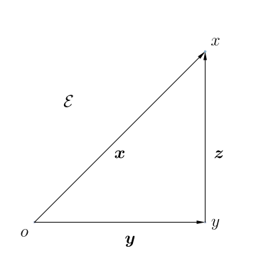
The shortest routes between points in $\mathcal{E}$ have important properties. For example, say $o$, $x$, $y$ are three points in $\mathcal{E}$, and say the shortest route to take to get from $o$ to $x$ is $\u{x}$, from $o$ to $y$ is $\u{y}$, and from $y$ to $x$ is $\u{z}$. It makes sense to add shortest routes. We can define the sum of the shortest route from $o$ to $y$ and the shortest route from $y$ to $x$ to be the shortest route from $o$ to $x$. As a consequence of this definition, the set of all shortest routes between all points in $\mathcal{E}$ form a vector space, and we denote it as $\mathbb{E}$, the Euclidean vector space. That is, $\u{x}$, $\u{y}$, and $\u{z}$ are vectors and they belong to $\mathbb{E}$.
Dimensional position vector
We call the shortest route to the point $x$ from $o$ the position vector of $x$, and denote it, as we have already been doing, as $\u{x}$. As previously discussed, all position vectors are vectors that belong to the vector space $\mathbb{E}$.
Physical quantities have units. For example, positions and distances in space have units of length – like meters, centimeters, etc. Specifically, the position vector $\u{x}$ of a particle $\mathcal{X}$ has units of length. We denote this statement by saying $[\u{x}]={\rm L}$, where $\rm L$ can be meters, etc.
Non-dimensional position vector
A vector space has a set of basis vectors, and we can write any vector as a linear combination of those vectors. Say $\left(\u{e}_1,\u{e}_2,\u{e}_3\right)$ is the set of basis vectors of $\mathbb{E}$.
As we have seen before, the position vector $\u{x}$ can be written as $x_i \u{e}_i$. In this representation we take $\u{e}_{i}$ to be the same physical quantities as $\u{x}$. Therefore, they have units. That is, $[\u{e}_{i}]={\rm L}$. We take $x_i$ to be dimensionless, i.e., they belong to $\mathbb{R}$, the set of real numbers. We symbolize the 3-tuple $(X_i)$, i.e., $(X_1,X_2,X_3)$, as $\usf{x}$. We take $\usf{x}$ to belong to the set of $3 \times 1$ matrices of real numbers. The set of $m\times n$ matrices of real numbers are denotes as $\mathcal{M}_{m,n}(\mathbb{R})$. We call $\usf{x}$ the non-dimensional position vector of $\mathcal{x}$.
Time, velocity, and acceleration vector spaces
Since the time $\u{t}$ is a physical quantity, it too has units; say $[\u{t}]=\rm T$, where $\rm T$ is a second, micro-second etc. We write $\u{t}=\tau \u{s}$, where $\u{s}$ is some characteristic time, i.e., $[\u{s}]=\rm T$, and $\tau$ is a real number, which we call non-dimensional time.
As the particle $\mathcal{X}$ moves around in $\mathcal{E}$ its position vector moves around in $\mathbb{E}$. We denote the position vector of $\mathcal{X}$ at the time instance $\u{t}$ as $\u{x}(\u{t})$. As before we can express $\u{x}(\u{t})$ as $x_i(\tau)\u{e}_i$. We call $\usf{x}(\tau):=\left(x_1(\tau),x_2(\tau),x_3(\tau)\right)$ the non-dimensional position vector of the particle $\mathcal{X}$ at the time instance $\tau$.
The velocity and acceleration of the material particle whose position vector at time $\u{t}$ is $\u{x}(\u{t})$ are
\(\begin{align} \u{V}(\u{t})&=\frac{d\u{x}(\u{t})}{d\u{t}},\\ \u{A}(\u{t})&=\frac{d^2\u{x}(\u{t})}{d\u{t}^2}, \end{align}\) respectively. The velocity vector $\u{V}(\u{t})$ and the acceleration vector $\u{A}(\u{t})$ are physical quantities, so they have units. Specifically, $[\u{V}(\u{t})]= {\rm L T^{-1}}$ and $[\u{A}(\u{t})]= {\rm L T^{-2}}$.
It can be shown that the set of all velocities that a material particle can possess form a vector space. So does the set of all accelerations that it can posses. We denote those vector spaces as $\mathbb{V}$, the velocity vector space, and $\mathbb{A}$, the acceleration vector space.
Let $\left(\u{v}_i\right)_{i \in (1,2,3)}$ and $(\u{a}_i)_{i\in(1,2,3)}$ be the sets of basis vectors of $\mathbb{V}$ and $\mathbb{A}$, respectively. Therefore, we can always express $\u{V}(\u{t})$ as $V_i(\tau)\u{v}_i$, where $V_{i}(\tau)$ are real numbers, and are called components of $\u{V}(\u{t})$ w.r.t $\u{v}_i$ , and $\u{A}(\u{t})$ as $A_i(\tau)\u{a}_i$, where $A_i(\tau)$ are (non-dimensional) real numbers, and are called the components of $\u{A}(\u{t})$ w.r.t. $\u{a}_i$. Here $\u{v}_i$ and $\u{a}_i$ are physical quantities, of the same character as $\u{V}(\u{t})$ and $\u{A}(\u{t})$, respectively. They consequently have units. Specifically, $[\u{V}_i]= {\rm L T^{-1}}$ and $[\u{A}_i]= {\rm L T^{-2}}$.
Then we call the $3\times 1$ matrix $\boldsymbol{\mathsf{V}}(\tau):=\left(V_{1}(\tau), V_{2}(\tau), V_{3}(\tau)\right)$ the non-dimensional velocity vector and $\boldsymbol{\mathsf{A}}(\tau):=\left(A_{1}(\tau),A_{2}(\tau),A_{3}(\tau)\right)$ the non-dimensional acceleration vector. It can be shown that
\(\begin{align} \boldsymbol{\mathsf{V}}(\tau)&=\frac{d\usf{x}(\tau)}{d\tau},\\ \usf{A}(\tau)&=\frac{d^2\usf{x}(\tau)}{d\tau^2}, \end{align}\) where, recall that, $\usf{x}(\tau):=\left(x_i(\tau)\right)_{i\in(1,2,3)}$.