Mechanics of Continua and Structures

Goal: To simulate the tests being conducted at Team Wendy using the framework of rigid body mechanics. Physics based computer simulations of head impact can aid in designing better helmets to protect the head.
Challenges:
Develop and implement a time integration algorithm that models the headform as a rigid body and is capable of simulating elastic collision between itself and another rigid body and has the following features.
- Conservation of energy in the absence of non-dissipative forces
- Conservation of energy during elastic impact
- Conservation of angular momentum in the absence of any applied torques
Technical work:
The most frequently used ordinary differential equations (ODE) time integrators for example, Runge-Kutta and Adams-Moulton schemes do not always preserve the important physics associated with rigid body motion. For example, in the absence of any applied forces or torques the rigid body motion is supposed to conserve both the total energy, and linear and angular momentum. However, if the usual integration schemes, such as the above mentioned ones, are used then the energy and the angular momentum in the simulation change with time. Another important aspect of the physics of rigid body motion is that it is necessary that the distance between any two points of the rigid body should remain constant during the simulations. However, the standard integration schemes do not respect this constraint.
We developed and implemented a geometric integration scheme, termed the Lie-Stormer–Verlet (LSV) integration scheme/algorithm. This scheme is based on the recently developed Lie-group geometric methods. We have implemented both an explicit and implicit version of this scheme. Both the explicit and implicit version of the LSV algorithm preserve the angular momentum in the absence of any applied torques. The explicit version is computationally cheaper than the implicit version. However, in the absence of any dissipative forces acting on the rigid body, the explicit version does not conserve the energy as well as the implicit version. The following equations summarize our rigid body dynamics model and the implicit LSV algorithm
The rigid body dynamics is modeled as follows,
\(\begin{align} \boldsymbol{x}_{t}(\boldsymbol{X})&=\boldsymbol{Q}_t\boldsymbol{X}+\boldsymbol{c}_t\\ \boldsymbol{V}_t(\boldsymbol{X})&= \dot{\boldsymbol{Q}}_t\boldsymbol{X}+\dot{\boldsymbol{c}}_t \label{eq:LagMatVel} \\ \boldsymbol{A}_t(\boldsymbol{X})&= \ddot{\boldsymbol{Q}}(t)\boldsymbol{X}+\ddot{\boldsymbol{c}}_t \label{eq:LagMatAccel} \end{align}\) where \(\boldsymbol{x}_t(\boldsymbol{X})\), \(\boldsymbol{V}_t(\boldsymbol{X})\), and \(\boldsymbol{A}_t(\boldsymbol{X})\) are, respectively, the position, velocity, and acceleration vectors of the material particle \(\boldsymbol{X}\) at the time instance \(t\). The tensor \(\boldsymbol{Q}_t\) is called the rotation tensor, and \(\boldsymbol{c}_t\) is called the translation vector. The physics of the rigid body dynamics that the distance between any two material points should not change during the rigid body’s motion is enforced by requiring that
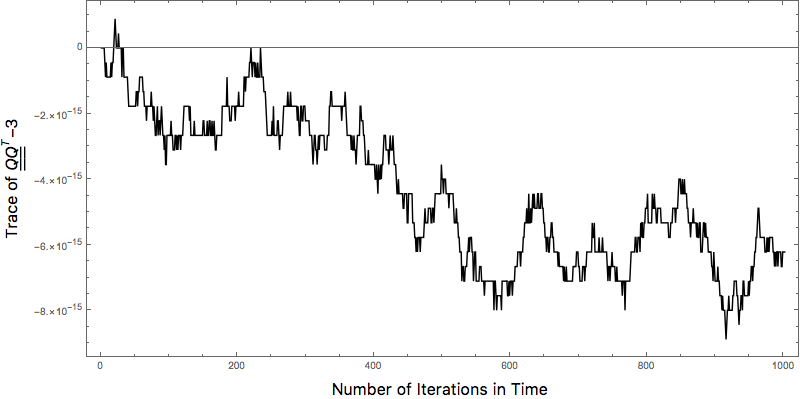
\(\begin{align} \boldsymbol{Q}^{\sf T}\boldsymbol{Q} &=\boldsymbol{I} \end{align}\) The above equation implies that the trace of \(\boldsymbol{Q}^{\sf T}\boldsymbol{Q}=3\).
The velocity field of the rigid body can also be written as
\(\begin{align} \boldsymbol{v}_t(\boldsymbol{x}) &=\boldsymbol{\omega}_t \times (\boldsymbol{x}-\boldsymbol{c}_t) +\dot{\boldsymbol{c}}_t, \end{align}\) where the vector \(\boldsymbol{\omega}_t\) is called the angular velocity vector.
For the implementation of the time integration algorithm we make use of the angular velocity tensor \(\star\boldsymbol{\omega}_t\), which is defined as
\[\begin{equation} \star\boldsymbol{\omega}_t = \boldsymbol{Q}_t^{\sf T}\dot{\boldsymbol{Q}_t} \end{equation}\]The operator \(\star(\cdot)\) is called the Hodge-Star operator. The angular velocity tensor \(\star\boldsymbol{\omega}_t\) is the Hodge-Dual of the angular velocity vector \(\boldsymbol{\omega}_t\).
The following equations summarize the implicit LSV algorithm.
\(\begin{align} \boldsymbol{\omega}_{n+1/2}&=\frac{1}{2} \boldsymbol{J}^{-1} e^{\Delta t\, (\star\boldsymbol{\omega_{n+1/2}})} \boldsymbol{J}\boldsymbol{\omega}_n+\boldsymbol{\omega}_n\\ \boldsymbol{Q}_{n+1}&=\boldsymbol{Q}_n e^{-\Delta t (\star\boldsymbol{\omega}_{n+1/2})}\\ \boldsymbol{\omega}_{n+1}&=\boldsymbol{J}^{-1} e^{\Delta t (\star\boldsymbol{\omega}_{n+1/2})}\boldsymbol{J}\boldsymbol{\omega}_n, \end{align}\) where \(\Delta t\) is the time step in the integration algorithm, \(\boldsymbol{Q}_{n+i}:=\boldsymbol{Q}_{(n+i)\Delta t}\), \(\boldsymbol{\omega}_{n+i}:=\boldsymbol{\omega}_{(n+i)\Delta t}\) \(i=1,~1/2\), \(\boldsymbol{J}\) is the inertia tensor, and \(\boldsymbol{J}^{-1}\) is the inverse of the inertia tensor. , i.e., \(\star \boldsymbol{\omega}_{n+1}\), \(\star \boldsymbol{\omega}_{n+1/2}\), \(\star \boldsymbol{\omega}_{n}\), are, respectively, the Hodge Duals of \(\boldsymbol{\omega}_{n+1}\), \(\boldsymbol{\omega}_{n+1/2}\), and \(\boldsymbol{\omega}_{n}\).
Accomplishments:
We have developed new computer software that successfully implements a implicit, time integration algorithm. This algorithm and the accompanying software has the following useful features.
- This implemented algorithm correctly preserves most of the important physics of rigid body dynamics. For example
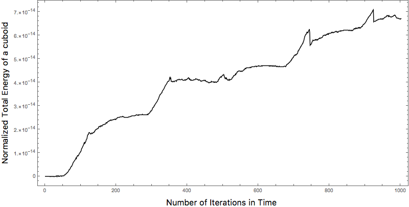
- Conserves the energy of the mechanical system in the simulation, up to machine precision, in the absence of non-dissipative forces
- Conserves energy of the mechanical system upto machine precision during elastic impact
- Conserves angular momentum of the mechanical system in the simulation, upto machine precision, in the absence of any applied torques
- The time integration algorithm has been implemented in two popular programming languages
- Matlab
- Mathematica
We have also written an API (application programming interface) that automatically converts the computer code that is written in Mathematica into a C-programming language code. In the future we plan on running the C-programming language based simulation on large-scale computer clusters.
- The time integration algorithm written in the Mathematica programming platforms can be deployed on the cloud. This would make the developed software accessible through the world wide web interface. Users can run the software through a simple web interface, through an internet browser, without the need for installing any special software.