Mechanics of Continua and Structures
Mechanics of 1D Continua:
Reduction of the shear deformable, finite deformation, 1D continua theory to a single nonlinear ODE
The equations derived by Wenqiang are as follows: \(\begin{align} \gamma &= \theta-\psi, \label{eq:def:gamma} \tag{1.1} \\ M &= \mathsf{E} \mathsf{I} \left(\psi'+\sec^2(\gamma)\gamma'\right), \tag{1.2} \label{eq:GEBM} \\ V&=-\mathsf{A} \mathsf{G}\tan(\gamma), \tag{1.3} \label{eq:1.3} \\ M'&=-V, \tag{1.4} \label{eq:1.4} \\ V&=-P_0\sin(\psi) \tag{1.5} \label{eq:1.5} \end{align}\)
From $\eqref{eq:1.3}$ and $\eqref{eq:1.5}$ we get that
\[\begin{align} \mathsf{A}\mathsf{G}\tan(\gamma)&=P_{0}\sin(\psi) \tag{2.1} \\ \tan(\gamma)&=\frac{P_0}{\mathsf{A}\mathsf{G}}\sin(\psi) \tag{2.2} \label{eq:Gamma_Psi} \end{align}\]Differentiating $\ref{eq:Gamma_Psi}$ we get
\[\begin{align} \sec^2(\gamma)\gamma'&=\frac{P_0}{\mathsf{A}\mathsf{G}}\cos(\psi)\psi' \tag{3.0} \label{eq:Gamma_Psi_Der} \end{align}\]Replacing the term $\sec^2(\gamma)\gamma’$ that appears in $\eqref{eq:GEBM}$ with the right hand side of $\eqref{eq:Gamma_Psi_Der}$, we get
\(\begin{align} M &= \mathsf{E} \mathsf{I} \left(\psi'+\frac{P_0}{\mathsf{A}\mathsf{G}}\cos(\psi)\psi'\right), \tag{1.2b} \label{eq:1.2b} \\ &=\mathsf{E} \mathsf{I} \left(1+\frac{P_0}{\mathsf{A}\mathsf{G}}\cos(\psi)\right)\psi', \tag{1.2c} \label{eq:1.2c}\\ \end{align}\) Differentiating $\eqref{eq:1.2c}$ we get \(\begin{align} M'&=\mathsf{E}\mathsf{I} \left(\left(1+\frac{P_0}{\mathsf{A}\mathsf{G}}\cos(\psi)\right)\psi'\right)' \tag{4.0} \label{eq:4.0} \end{align}\)
Substituting $V$ in $\eqref{eq:1.4}$ with the right hand side of $\eqref{eq:1.5}$ and $M’$ in $\eqref{eq:4.0}$ with the right hand side of $\eqref{eq:4.0}$ we get
\[\begin{align} \mathsf{E}\mathsf{I} \left(\left(1+\frac{P_0}{\mathsf{A}\mathsf{G}}\cos(\psi)\right)\psi'\right)' &=P_0 \sin(\psi) \label{eq:5.0} \tag{5.0} \end{align}\]Introducting the non-dimensional variable $\hat{s}=s/\ell$, where $\ell$ is an arbitrary unit of length
\[\begin{equation*} \frac{d(\cdot)}{ds}\to\frac{1}{\ell}\frac{d(\cdot)}{d\xi} \end{equation*}\]in $\eqref{eq:5.0}$ we get
\[\begin{align} \left(\left(1+\frac{P_0}{\mathsf{A}\mathsf{G}}\cos(\psi)\right)\psi'\right)' &=\frac{P_0 \ell^2}{\mathsf{E} \mathsf{I}} \sin(\psi) \label{eq:6.1} \tag{6.1} \end{align}\]Defining
\[\begin{align} \hat{P}_0&:=\frac{P_0 \ell^2}{\mathsf{E} \mathsf{I}}\\ \hat{\mu}&:=\frac{G A\ell^2}{\mathsf{E} \mathsf{I}} \end{align} \label{def.2} \tag{def.2}\]Equation $\eqref{eq:6.1}$ can be written as
\[\begin{align} \left(\left(1+\frac{\hat{P}_0}{\hat{\mu}}\cos(\psi)\right)\psi'\right)' &=\hat{P}_0\sin(\psi) \end{align}\]we get
\[\begin{align} \left(\left(1+\hat{P}_{0}\cos(\psi)\right)\psi'\right)' &=\hat{P}_0\hat{\mu} \sin(\psi) \label{eq:7.0} \tag{7.0} \end{align}\]The nonlinear differential equation $\eqref{eq:7.0}$ is subject to the boundary conditions
\(\begin{align} \psi(0)&=0, \label{eq:7.1a} \tag{7.1} \\ \psi'(\hat{L})&=0, \label{eq:7.1b} \tag{7.2} \end{align}\) where
\[\begin{align} \hat{L}&:=\frac{L}{\ell} \tag{def.3} \label{def.3} \end{align}\]Failure stresses at the root
\[\begin{align} M&=\mathsf{E} \mathsf{I} \left(\psi'+\sec^2(\gamma)\gamma'\right)\\ \frac{M}{\mathsf{E} \mathsf{I}}&= \left(\psi'+\sec^2(\gamma)\gamma'\right)\\ \frac{M }{\mathsf{E} \mathsf{I}}&= \left(1+\frac{\hat{P}_0}{\hat{\mu}}\cos(\psi)\right)\psi' \end{align}\]Multiple solutions and their energies
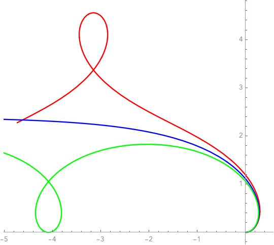
- Different shapes for same force
Total potential energy
\[\begin{align} \hat{\Pi}:=\frac{\Pi\ell}{\mathsf{E}\mathsf{I}} \end{align}\] \[\begin{align} \hat{\Pi}= \frac{1}{2} \int_{0}^{\hat{L}} \left( 1+\hat{P}_0\cos(\psi) \right)^2\psi'^2\, d\hat{s} + \frac{1}{2} \hat{P}_0^2\hat{\mu} \int_{0}^{\hat{L}} \sin^2(\psi)\, d\hat{s} - \hat{P}_0\hat{\mu} \int_{0}^{\hat{L}} (\cos(\psi)-1)\, d\hat{s} \end{align}\]The energies of the red, blue, and green deformed configuration are, respectively, -5.39304, -11.0318, -4.91333. The relatively straight shape has the lowest energy.
Numerical solution using the shooting method
See this mathematics code for a sample numerical solution of the equation $\eqref{eq:7.0}$, subject to the boundary conditions $\eqref{eq:7.1a}$ and $\eqref{eq:7.1b}$.
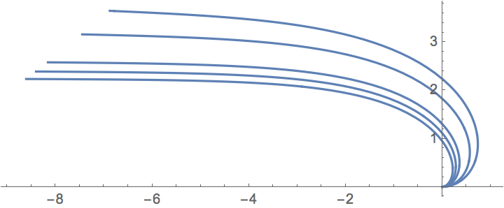
Some sample results from this mathematics code.
Remark: For a given set of boundary conditions, there are several solutions to the nonlinear differential equation. We need to slightly perturb the boundary conditions or guide the solution through the initial guess to numerically arrive at the solution that has the physical characteristics (e.g., containing a loop) that we are most interested.